his section is of academic significance. To derive a preconditioner
from asymptotic decomposition is a very natural attempt. The author feels
compelled to document it even so the final result could be guessed. The reader
may skip this section without consequence.
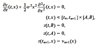
According to the section
(
Reduction
to system of linear algebraic equations for q=1
), we need to solve the
equation
 where
where
 Thus, we transform
 into the set of coefficients
 such
that
 is an approximation to the solution
 of the
problem
 taken at
 :
:

In the section
(
Asymptotic
expansion for Black equation
) we calculated an approximate solution to the
problem
 in the
form
 Thus we have an explicit transformation

 where
where
 is close to
 .
We use such transformation to construct a preconditioner
 for the
step
 of the chain
 .
.
It is essential that
 are constructed as piecewise quadratic functions in
 ,
see the sections
(
Calculation of boundary
scaling functions
),
(
Calculation
of approximation spaces in one dimension II
). Thus, the first derivative
is continuous and piecewise linear function and the second derivative is a
piecewise constant function. We do not reach a situation when we would have to
keep track of delta functions. We can apply facilities of PiecewisePoly
library (see the section
(
Manipulation
of localized piecewise polynomial functions
)) without additional
modification. It also helps to do integration by part to even out
differentiation.
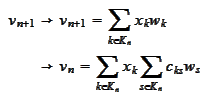
For every
 consider
the
transformation
 where the
 might be outside of
span
 .
The sum should be understood as a projection. We put together the matrix
 Hence, the semi-solution
 would
act
 Thus
Thus
 The
The
 is represented by

 where
where
 is the
 -Gram
matrix
 and
and
 is a column
 .
.
Thus we arrive to the
chain
 Therefore, we
set

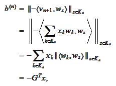
The projection in the above summary is calculated as follows.
We introduce the convenience notation
 :
:
 Then the coefficients
 come from the
relationships
 for the
 scalar product
 .
Thus
 or
or
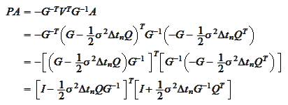
 The expression for the preconditioner
is
 thus
thus

It remains to improve the calculation of
 :
:
 where the functions
 are piecewise polynomials in
 vanishing at the ends of integration interval. We integrate by
parts:
 and arrive to the same expression we already use when constructing the matrix
 .
Thus

 while the matrix
 is given
by
 Hence the preconditioned matrix
is
 The matrix
 is
symmetric.

|