e apply recipes of the section
(
Reduction
to system of linear algebraic equations
) to the problem
(
Example strong Black problem
2
).
We introduce the time
mesh
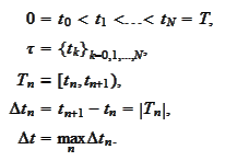
The location of the points
 is to be chosen according to the statement
(
Convergence of
discontinuous Galerkin technique
) and will be addressed in the section
(
Adaptive time step for
Black PDE
).
First, we apply results of the section
(
Decomposition
of payoff function in one dimension section
) to the function
 of the problem (
Example strong
Black problem 2
). Thus, we have a wavelet basis
 and we start from
decomposition
 for some index set

According to the results around the formula
(
Matrix of discontinuous
Galerkin
), we perform a single time step transformation by solving the
equation
 where we introduce double indexes
 ,
,
 ,
,
 is a column
 ,
,
 is a
matrix
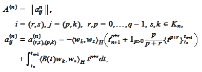
 For the present problem, the operator
 does not have
 -dependency.
Hence
 and
and
 where the functions
 are second degree piecewise polynomials constructed to be in
 .
The column
 comes from previous step or input
data:
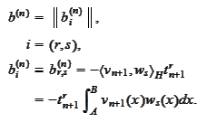 Thus, for
 ,
we put
 and for
 the
the
 is taken from the previous step.
We introduce the
notations
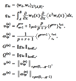 Then
Then
 We arrange indexes
 by changing the spacial indexes
 before changing the time indexes
 .
Then the matrix
 has block structure. For
 we
get

For any matrixes
 and
and
 ,
we introduce the notation
"
 ":
":
 Note
that
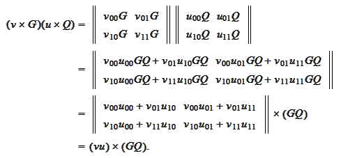
We
get
 where the last line is valid for all
 .
.
For
 we
calculate
 Let
Let
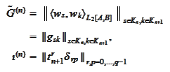 then
then
 We
obtain
 Note that
 is a strongly diagonal matrix and
 is a well conditioned matrix. We act on the last equation by
 and
obtain

The summary above shows that if the operator
 is
is
 -independent
then we can solve the problem with
 using the same manipulations as in the case
 without noticeable increase in memory requirements. The space and time parts
of the problem may be processed separately. This observation extends to a
situation when there is multiplicative separation of space and time dependent
expressions in the PDE, for
example

|