pplication of finite
element technique to multidimensional problems suffers from curse of
dimensionality. Our silver bullet for such curse is combined use of sparse
tensor product (see the section
(
Sparse tensor product
)), high
order wavelets (see the section (
Wavelet
analysis
)) and adaptive grid (see the section
(
Adaptive approximation
)).
The scaling functions
 ,
,
 calculated in the section
(
Calculation of scaling
functions
) are approximations. Recall that we perform the procedure
calculated in the section
(
Calculation of scaling
functions
) are approximations. Recall that we perform the procedure
 starting from some
 and stop after a finite number of steps
 .
We use
.
We use
 ,
,
 as approximations for
 .
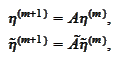
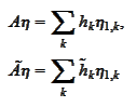
Hence
.
Hence
 instead of the desired relationship (
Scaling
equation
):
instead of the desired relationship (
Scaling
equation
):
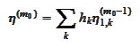
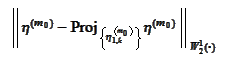
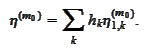 Therefore, we would like to project
 on linear span of
 .
The size of the
difference
.
The size of the
difference
 is indication of success of the procedure.
So far we have calculated wavelets on the interval (see the sections
(
Adapting
scaling function to the interval [0,1]
) and
(
Adapting wavelets
to the interval [0,1]
)). If we attempt to use the functions
 ,
,
 as a basis of sparse tensor product then we must be able to evaluate
projection
as a basis of sparse tensor product then we must be able to evaluate
projection
 for all
 and the difference between the projection and the original in
 norm should be small. For calculation of the projection to be affective, the
Gram matrix
norm should be small. For calculation of the projection to be affective, the
Gram matrix
 must have a low condition number for all
 .
The script tCondNumber.py shows that the Gram
matrix
.
The script tCondNumber.py shows that the Gram
matrix
 has condition number below 6 for any
 .
Therefore, our goal is to pick boundary functions that do not significantly
increase the condition number of the whole matrix. The boundary wavelets are
chosen with the same consideration.
.
Therefore, our goal is to pick boundary functions that do not significantly
increase the condition number of the whole matrix. The boundary wavelets are
chosen with the same consideration.
|
