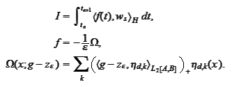
n this section we
consider time discretization for the
expression
 The
The
 depends on a function
 that comes from the equation where
 participates. Theory of numerical methods for ODE have a similar problem and
an effective solution. We review the theory.
Consider the
ODE
 The time evolution happens backwards from
 to
to
 .
Taylor decomposition applies to
 and
and
 in all arguments. The
 is an input value.
We introduce a time mesh
 and a mesh function
 defined
recursively
 Thus
Thus
 We proceed to estimate the magnitude of the difference
 for all
 .
We
calculate
 We subtract and use
 :
:

For a general time step we
calculate


 thus
thus
 Then
Then
 assuming that all
 are of generally the same magnitude.
Following recipes of Runge-Kutta technique, we introduce a better
approximation
 as
follows:
 We seek parameters
 that deliver the smallest difference
 .
.
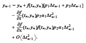
We calculate the evolution equation for
 :
:
 Therefore

|
|
(Evolution of y)
|
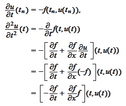
We use Taylor expansion for
 :
:
 and substitute the time derivatives using the defining equation for
 :
:
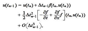
 and put all
together:

|
|
(Evolution of u)
|
By comparing the formulas (
Evolution of y
) and
(
Evolution of u
), we
require
 We
set
 then
then


At initial time step
 we get
 and then the higher order propagates.
The crucial requirement is smoothness of
 .
In our case, see the expression for
 ,
the function
 would jump. Hence, the expression
 is not small for those values of
 and
and
 on opposite sides of the jump. Given the nature of the problem, it would be
typical.
One might try to replace the operation
 within the function
 with some smooth function with similar
properties:
 The function
 must be zero where
 is zero. But then, to be smooth, it must increase gently on the other side of
the
 area. One could argue that it would hurt the purpose of the penalty term,
dampening convergence of the procedure and requiring higher
 .
But then, one could also argue that this is what we want: we are not certain
about desired strength of the penalty term, thus, we would like to employ a
graduate procedure of high order.
In the following chapter
(
Smooth version of
penalty term
) we will point out a reason why, in fact, we must do such
modification.
|