he procedure of the section
(
Mix
of backward induction and penalty term approaches
) is implemented in the
script soMix1.py located in the directory OTSProjects/python/wavelet2.
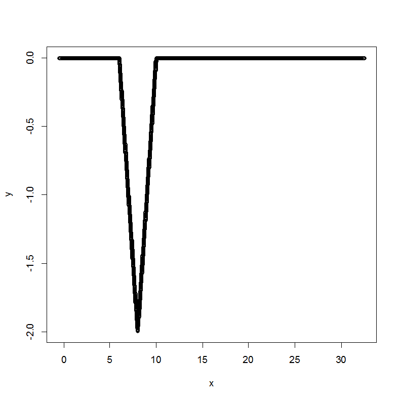
The payoff function
 .
.
|
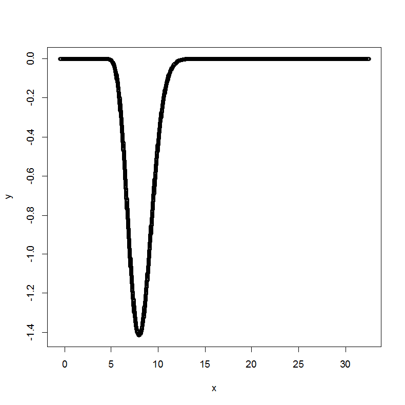
Evolution via mean reverting
equation for
 :
:
 .
No optimization.
|
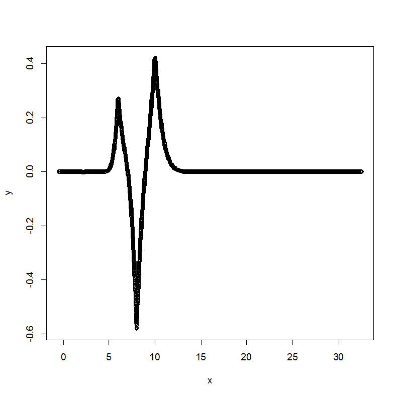
Plot of
 .
.
|
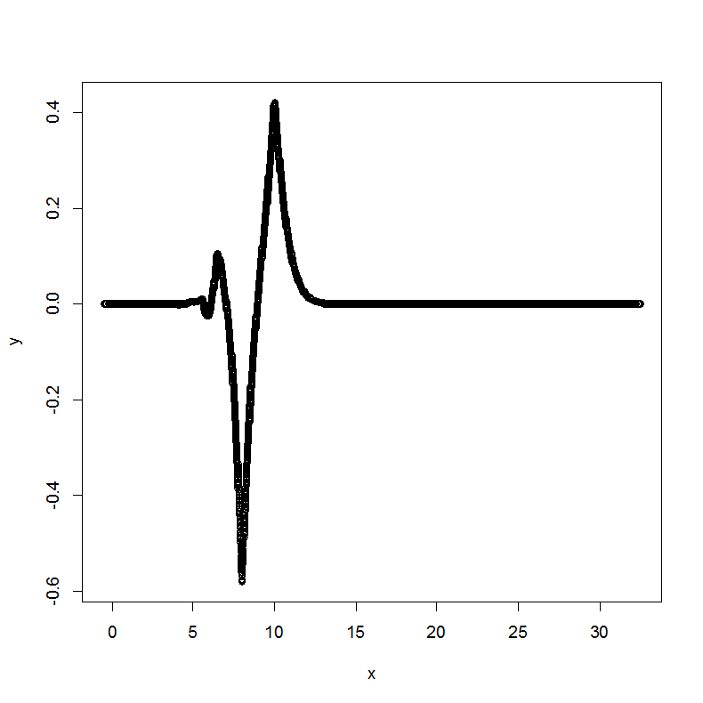
Plot of
 for scale of probing hut functions
 .
The
.
The
 term is localized to left side only. Two probing functions are used.
|
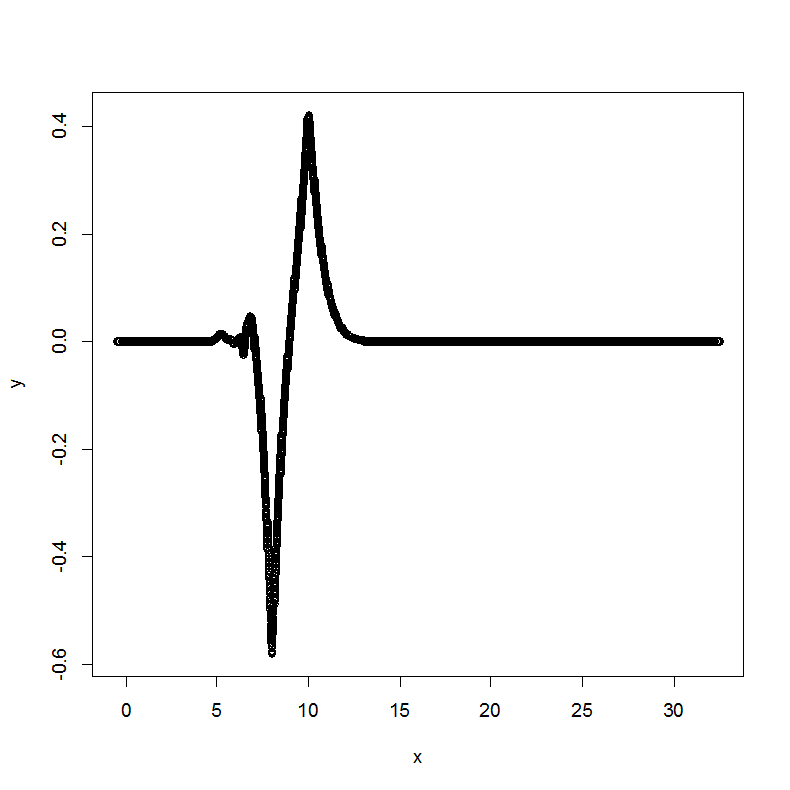
Plot of
 for scale of probing hut functions
 .
The
.
The
 term is localized to left side only. 8 probing functions are used.
|
We note the following.
(1). The procedure is not effective at the boundary. This is so because we
cannot place probing functions at the boundary to avoid overshooting. See the
previous section
(
Mix
of backward induction and penalty term approaches
).
(2). We pick up negative values in the middle of the corrected interval. This
happens for two reasons:
(2a). At the edge of the plot of difference
 the absolute value of derivative
 might exceed absolute value of derivative of the probing function.
(2b). The
 is a projection of probing function on the wavelet basis
 .
The basis is adapted to
 and
and
 and is not adapted to represent the probing function.
(3). In process of the optimization procedure we have to do considerable
number of evaluations of both objective function and constraints.
For these reasons we make yet another modification of the procedure.
|