e continue
considerations of the previous section.
We are solving a slightly non-linear system of algebraic equations using a
Newton technique and we are having problems because of limitations on area of
convergence. The next most effective relevant numerical technique is
Runge-Kutta technique. In order to apply it, perhaps in combination with the
Newton procedure, we need a continuous parameter that would produce a Cauchy
problem with smooth RHS. The idea is to make a Runge-Kutta step, then improve
using Newton and then do Runge-Kutta again and so fourth.
The system of equations is
 with
with

The continuous parameter that we need for our Cauchy problem is reversed time.
Let
 Then
Then
 and
and
 solves the equation for
 .
We rewrite the
equation:
 and differentiate with respect to
 :
:
 or
or
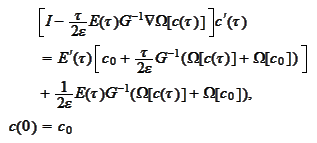
 and we obtain a Cauchy problem. We now have the function
 that solves both Cauchy problem and algebraic problem for all
 .
We apply Runge-Kutta and Newton interchangeably, as discussed above.
Next, we calculate the components.
The term
 was considered in the previous section.
According to the summary
(
Summary for mean
reverting equation in case
q=1
),
 Thus
Thus
 However, such approach requires calculation of
 for variety of
 .
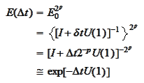
Instead, we do exponentiation. We select a
 ,
a power
 and
calculate
 This
way
 for reasonably large
 .
Such
 has multiplicative
property
 which is especially useful in present situation. We
have

The procedure is implemented in the script soCauchy2.py within the directory
OTSProjects/python/wavelet2. We are able to make reasonably small time steps
without stability and divergence issues. However, the procedure exhibits
uncomfortable level of sensitivity to the control parameters
 ,
,
 and scale of probing functions. In the following section we discuss reasons of
such sensitivity and propose an improved procedure.
|