e calculate
the matrix
 as described in the summary
(
Summary for mean
reverting equation in case q=1
) and then apply manipulations of the
summary
(
Summary
for Black equation in case q=1, inverted matrix
). We compare the results
with the formula
(
Analytical
solution for mean reverting equation
). The difference is the fourth digit,
consistently with the precision of the section
(
Rebalancing wavelet basis
section
) that we use when removing insignificant basis functions.
All scripts are located in the directory OTSProjects/python/wavelet2. The
localization and gram matrix calculations are implemented in the scripts
mrGram.py and mrMrGram.py. Initial grid calculation, see the section
(
Decomposition
of payoff function in one dimension
), is in the script mrGrid.py. The
whole procedure is put together in the script mrFinal.py.
We calculate solution for the following
parameters:
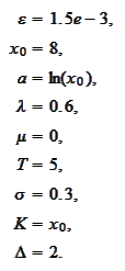 Initial grid consists of 76 basis points but then calculations of the section
(
Rebalancing wavelet basis
section
) reveal that we need no more than 42.
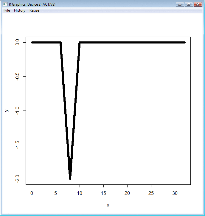
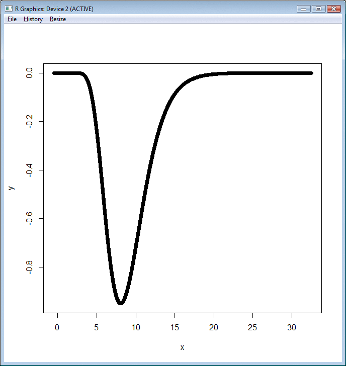
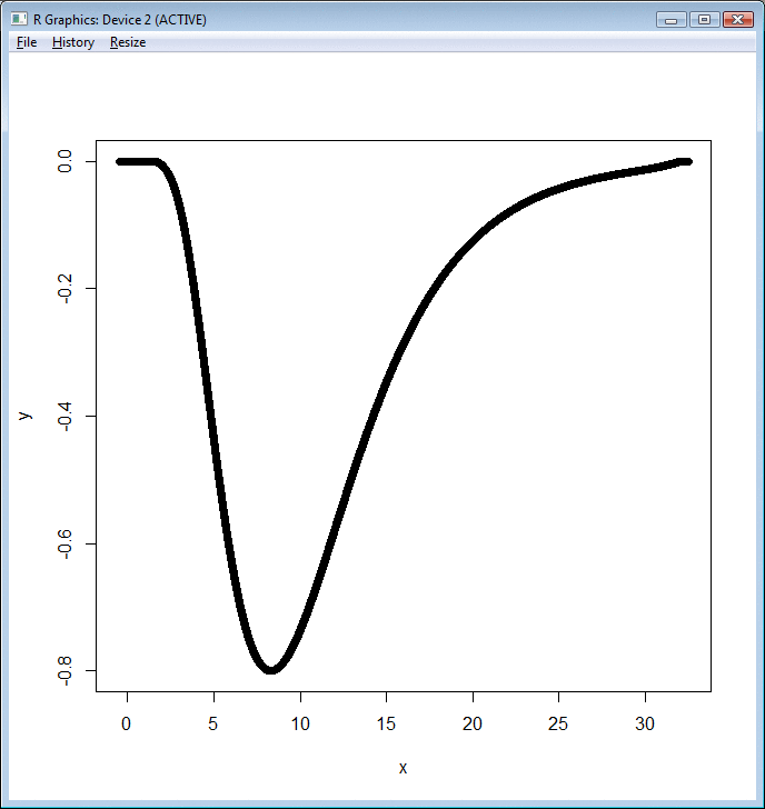
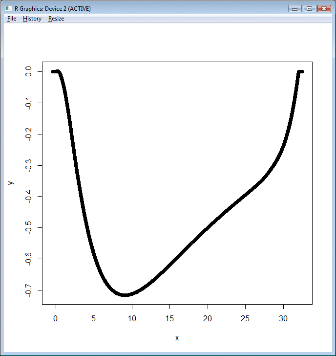
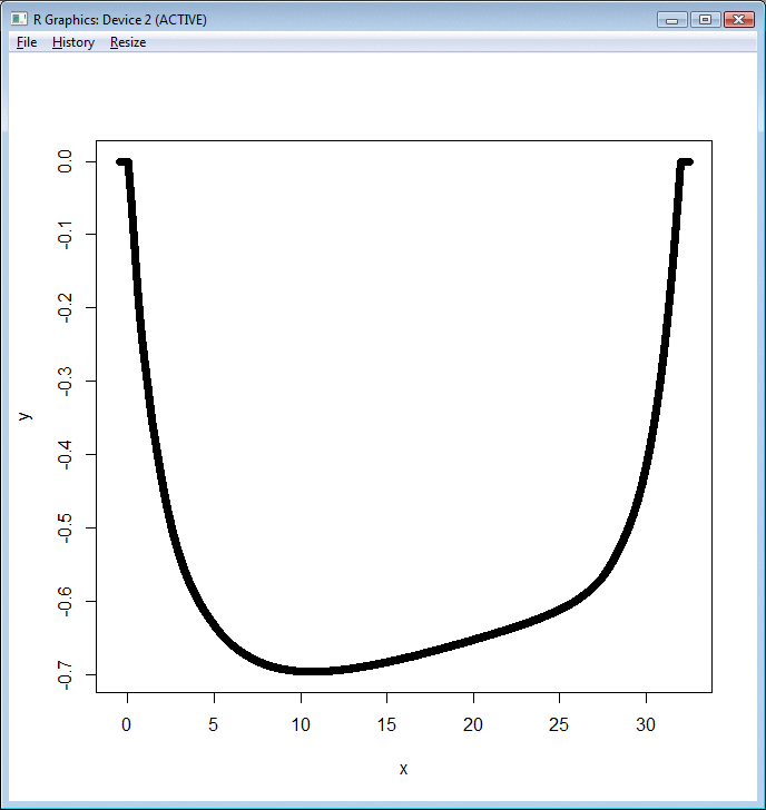
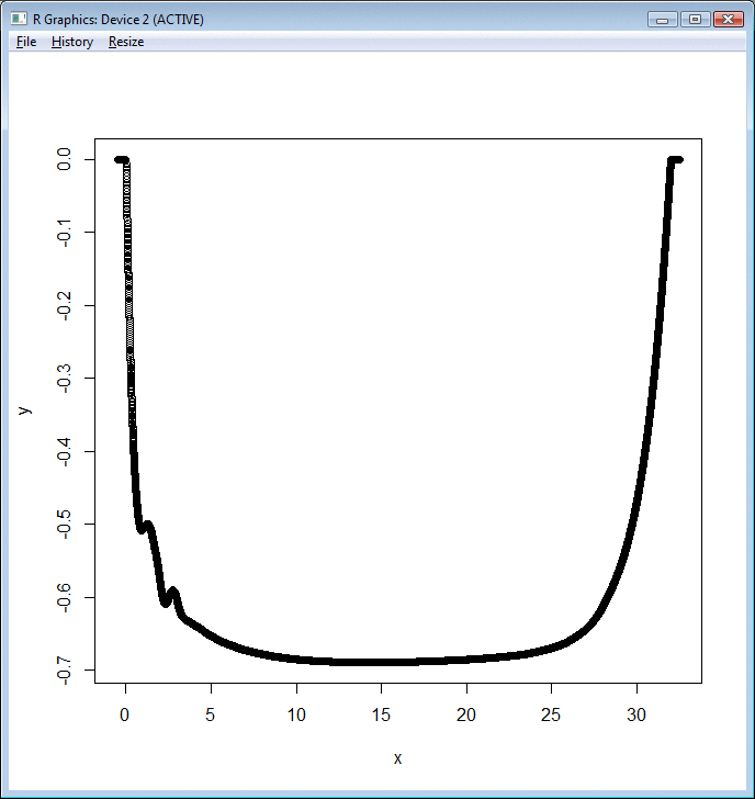
The following figures (
Mean reversion 0
) to
(
Mean reversion 5
) depict evolution of the
solution as time
 changes from
 to
to
 .
The slight instability on the figure (
Mean
reversion 5
) indicates that we do not have enough basis functions at the
area where the solution changes fast. Comparison with the analytical solution
(
Analytical
solution for mean reverting equation
) indicates that the precision in the
central area remains good.
Plot of
 .
.
|
Plot of
 .
.
|
Plot of
 .
.
|
Plot of
 .
.
|
Plot of
 .
.
|
Plot of
 calculated with 24 basis functions.
|
|