Quantitative Analysis
Parallel Processing
Numerical Analysis
C++ Multithreading
Python for Excel
Python Utilities
Services
Author
Printable PDF file
I. Basic math.
II. Pricing and Hedging.
III. Explicit techniques.
IV. Data Analysis.
V. Implementation tools.
VI. Basic Math II.
VII. Implementation tools II.
1. Calculational Linear Algebra.
2. Wavelet Analysis.
A. Elementary definitions of wavelet analysis.
B. Haar functions.
C. Multiresolution analysis.
D. Orthonormal wavelet bases.
E. Discrete wavelet transform.
F. Construction of MRA from scaling filter or auxiliary function.
G. Consequences and conditions for vanishing moments of wavelets.
H. Existence of smooth compactly supported wavelets. Daubechies polynomials.
I. Semi-orthogonal wavelet bases.
a. Biorthogonal bases.
b. Riesz bases.
c. Generalized multiresolution analysis.
d. Dual generalized multiresolution analysis.
e. Dual wavelets.
f. Orthogonality across scales.
g. Biorthogonal QMF conditions.
h. Vanishing moments for biorthogonal wavelets.
i. Compactly supported smooth biorthogonal wavelets.
j. Spline functions.
k. Calculation of spline biorthogonal wavelets.
l. Symmetric biorthogonal wavelets.
J. Construction of (G)MRA and wavelets on an interval.
3. Finite element method.
4. Construction of approximation spaces.
5. Time discretization.
6. Variational inequalities.
VIII. Bibliography
Notation. Index. Contents.

Calculation of spline biorthogonal wavelets.


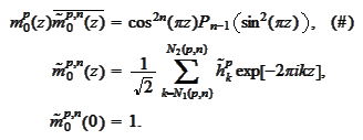
n this section we implement the procedure of the proposition ( Existence of biorthogonal compactly supported wavelets ) by taking $\phi=\tilde{B}_{p}$ (see the definition ( Spline functions )) for some $p\in\QTR{cal}{N}$ . According to the proposition ( Properties of spline functions )-4, MATH We seek MATH to satisfy MATH

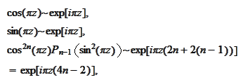
For fixed $p$ , $n$ the MATH are selected to insure that the highest powers of MATH and MATH would be the same on both sides of the equation $\left( \#\right) $ . Therefore, we calculate the highest power of MATH as follows MATH MATH thus MATH or MATH We calculate the highest power of MATH : MATH MATH thus MATH or MATH

Remark

Note that the number of terms in the sequence $\tilde{h}_{k}^{p}$ is MATH and the number of terms in the sequence $h_{k}:$ MATH is MATH For purposes of the section ( Adapting GMRA to interval [0,1] ) we need MATH Thus, we need MATH or MATH Therefore, to have $n$ vanishing moments and the same supports for $\phi$ , $\tilde{\phi}$ it suffices to introduce MATH and MATH with the following lengths: MATH MATH

Remark

(Unsuitability of spline wavelets) Note that in the expression $\left( \#\right) $ the terms MATH and MATH partially cancel out. This means that instead of MATH the MATH and MATH have representations MATH for some MATH . As a result, we cannot have both equal supports for $\phi,\tilde{\phi}$ and equal number of vanishing moments for $\psi$ and $\tilde{\psi}$ . Therefore, we are forced to seek alternative approach to factorization of the expression MATH in the following sections.

Remark

(Unsuitability of spline wavelets 2)Obtained this way wavelets are not symmetrical with respect to regularity. The $\phi$ is set to be a spline. The function $\tilde{\phi}$ is wildly oscillating.

The procedure is implemented by the following Mathematica script. The results agree with the Python's pywt module and [Walnut] up to cubic spline wavelets (p<=2,n<=5).

n=2

p=2*n-2

CC[k_, n_] := Binomial[n, k]

Pnm1[n_, y_] := Expand[Sum[CC[k, 2*n - 1]*y^k*(1 - y)^(n - 1 - k), {k, 0, n - 1}]]

N1[p_,n_]:= p-2*n+2

N2[p_,n_]:= 2*n-1

m0[p_, x_] :=(1/2*(1+Exp[-2*Pi*I*x]))^(p+1)

M0[p_,n_,x_] := 1/Sqrt[2]*Sum[H[k]*Exp[-2*Pi*I*k*x], {k, N1[p,n],N2[p,n]}]

LHS[p_,n_,z_] := m0[p, z]*Conjugate[M0[p,n, z]]

RHS[n_, z_] := (Cos[Pi*z])^(2*n)*Pnm1[n, (Sin[Pi*z])^2]

Cond[p_,n_, z_] := Expand[TrigToExp[RHS[n, z]]] - TrigToExp[ComplexExpand[LHS[p,n,z]]]

x1 = Cond[p,n, z]

d=4*n

x2 = Collect[x1*Exp[d*I*Pi*z], Exp[I*Pi*z]]

L=CoefficientList[x2, Exp[I*Pi*z]]

eqs=Map[Function[x, x == 0], L]

eqs2 = Map[Function[x, Im[H[x]] == 0], Range[N1[p,n],N2[p,n]]]

eqs3 = { M0[p,n,0]==1 }

vars = Map[Function[x, H[x]], Range[N1[p,n],N2[p,n]]]

solA=NSolve[Join[eqs, eqs2, eqs3], vars]

m0B[p_, x_] := 1/Sqrt[2]*Sum[h[k]*Exp[-2*Pi*I*k*x], {k, 0,p+1}]

CondB[p_,z_] := Expand[m0[p,z]-m0B[p,z]]

x1 = CondB[p,z]

x2 = Collect[x1, Exp[-I*Pi*z]]

L=CoefficientList[x2, Exp[-I*Pi*z]]

eqs=Map[Function[x, x == 0], L]

eqs2 = Map[Function[x, Im[h[x]] == 0], Range[0,p+1]]

vars = Map[Function[x, h[x]], Range[0,p+1]]

solB=NSolve[Join[eqs, eqs2], vars]

{solA,solB}


Notation. Index. Contents.


Copyright 2007