e build on results of the
section (
Calculation
of biorthogonal wavelets
) and use technique of the section
(
Adapting MRA to the
interval [0,1]
).
Therefore, according to the proposition
(
Reproduction of polynomials
4
),
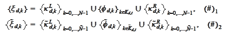
According to the definition (
Dual
wavelets
),
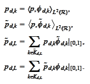
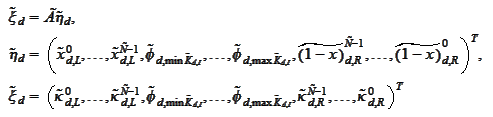
We introduce the notations
 ,
,
 ,
,
 ,
,
 ,
,
 ,
,
 ,
,
 ,
,
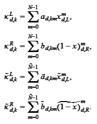
 similarly to the section
(
Adapting MRA to the
interval
[0,1]
):
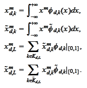
similarly to the section
(
Adapting MRA to the
interval
[0,1]
):
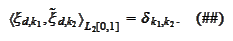
 According to the condition
(
Biorthogonal scaling
functions
)-2,
According to the condition
(
Biorthogonal scaling
functions
)-2,
Condition
(Sufficiently fine scale 2) We assume
that the parameter
 is sufficiently large so
that
is sufficiently large so
that

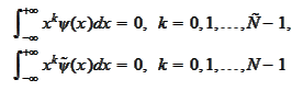
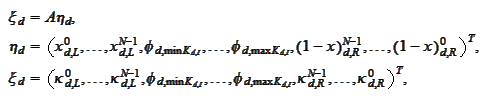
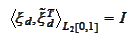
For a polynomial
 we
have
we
have
 We introduce the
notation
We introduce the
notation
 In
particular,
In
particular,
Definition
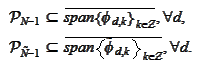
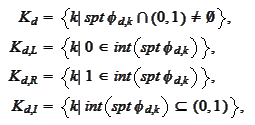
([0,1]-adapted GMRAs) We define the
spaces
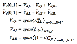
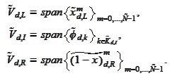
We proceed to construct biorthogonal bases for
 ,
,
 for each
 .
.
Let
 We choose
 ,
,
 ,
,
 ,
,
 to
satisfy
to
satisfy
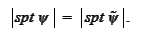
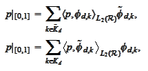
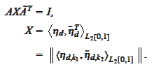
We represent the relationships
 and
and
 as
as
 for some matrixes
 chosen to satisfy
 :
:
 so
that
so
that
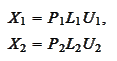
If
 then
then
 is a square matrix of the
form
is a square matrix of the
form
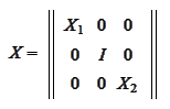 with some square matrixes
 The LU decomposition may be applied separately to the matrixes
 :
:
 for some permutation matrixes
 ,
lower triangular matrixes
,
lower triangular matrixes
 and upper triangular matrixes
 .
The
choice
.
The
choice
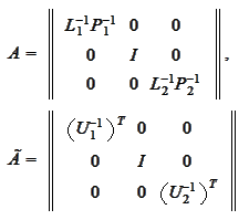 delivers one possible solution.
|