n this chapter we consider a
technique that extends the finite elements (discussed in the chapter
(
Finite elements
)) to financial
instruments involving stochastic optimal control (American feature). The
reference is
[Bensoussan]
.
We previously introduced a backward induction and Bellman equation in the
sections (
Backward induction
) and
(
Bellman equation
). We now study
variational inequalities because direct application of Bellman equation is not
possible in combination with Finite Element technique. Indeed, when conducting
Finite Element calculations, we evolve a vector of coordinates with respect to
some finite element basis. Bellman equation requires us to continuously take
maximum among some function values. We would like to avoid assembling and
disassembling basis decompositions on every time step. In multidimensional
situation such operation is not even feasible.
To see how a stochastic control problem may lead to a variational inequality
consider first the following problem of evaluation of
 :
:
 where the
 is the standard Brownian motion, the
 is the first exit time of the process
 from
from
 for
for
 ,
,
 is a bounded set with smooth boundary and
 is a function
 and
and
 ,
,
 .
We saw in the section
(
Representation
of solution for elliptic PDE using stochastic process
) that the
 solves the following
problem
 We apply such result in context of the section
(
Optimal stopping time
problem
). We modify the task to find the function
 defined by the
relationships
 Combining the calculations of the sections
(
Representation
of solution for elliptic PDE using stochastic process
) and
(
Optimal stopping time
problem
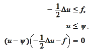
) we conclude that such
 solves the following free boundary
problem
 almost everywhere in
 and
and

Observe that the above problem may be rewritten
as

|
|
(Variational inequality example)
|
where the bilinear form
 (compare with the section (
Elliptic PDE
section
)) is given
by
 and the class of functions
 is defined as

To see the equivalence of the two formulations consider the area where
 .
We can find two functions
 and
and
 from
from
 such that
 and
and
 .
Then
 for
for
 implies
 .
One the other hand, in the area where
 we always have
 is nonpositive for
 and thus
 implies
 .
.
|