Quantitative Analysis
Parallel Processing
Numerical Analysis
C++ Multithreading
Python for Excel
Python Utilities
Services
Author
Printable PDF file
I. Basic math.
II. Pricing and Hedging.
III. Explicit techniques.
IV. Data Analysis.
V. Implementation tools.
VI. Basic Math II.
VII. Implementation tools II.
1. Calculational Linear Algebra.
A. Quadratic form minimum.
B. Method of steepest descent.
C. Method of conjugate directions.
D. Method of conjugate gradients.
E. Convergence analysis of conjugate gradient method.
F. Preconditioning.
G. Recursive calculation.
H. Parallel subspace preconditioner.
2. Wavelet Analysis.
3. Finite element method.
4. Construction of approximation spaces.
5. Time discretization.
6. Variational inequalities.
VIII. Bibliography
Notation. Index. Contents.

Recursive calculation.


roposition

(Recursive calculation) Suppose MATH then for any $x_{0}$ and $z$ the sequence MATH MATH converges MATH to the solution $x^{\ast}$ of the equation

MATH (Recursive equation)

Proof

We subtract the relationships MATH and obtain MATH Hence MATH

There following are (at least) two ways one can arrive to the equation ( Recursive equation ) starting from the equation ( Linear equation ).

Proposition

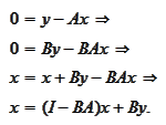
(Reduction scheme 1) Suppose a non-singular matrix MATH has the decomposition MATH with an invertible matrix $A_{1}$ then the solution $x^{\ast}$ of the equation ( Linear equation ) also satisfies the equation MATH

Proof

We calculate

MATH

Proposition

(Reduction scheme 2) Let MATH are two non-singular matrixes then the solution $x^{\ast}$ of the equation ( Linear equation ) also satisfies the equation MATH

Proof

We calculate MATH

For both propositions ( Reduction scheme 1 ) and ( Reduction scheme 2 ) we want to almost invert the matrix of the original problem ( Linear equation ). The same is true for the preconditioner $B$ of the section ( Preconditioning ). It appears that preconditioner $B$ the section ( Preconditioning ) may be used as a matrix $B$ of the proposition ( Reduction scheme 2 ), provided that the condition MATH holds. The reverse statement is also true. However, the preconditioned conjugate gradient technique converges faster as the following proposition shows.

Proposition

Assume that MATH is symmetric, MATH is symmetric positive definite and MATH then MATH is symmetric positive definite, MATH (see the formula ( Condition number ) for definition of $\kappa$ ) and MATH (Compare with the proposition ( Convergence of conjugate gradient method )).

Proof

First, we prove that $B$ is positive definite. Assume the contrary: there exists an eigenvector $v$ of $B$ with non positive eigenvalue $\lambda_{v}$ . Then MATH The term MATH is positive by assumption of the proposition. MATH Then we cannot have $\left( \&\right) $ . We arrive to a contradiction.

Next, we estimate MATH . By $\left( \&\right) $ we have MATH Hence MATH Finally, we estimate MATH . The function MATH is increasing for $x>1$ . Indeed, MATH Hence, MATH MATH


Notation. Index. Contents.


Copyright 2007