ccording to the proposition
(
Convergence of conjugate
gradient method
), the procedure of the summary
(
Conjugate gradients
) converges
significantly better when
 and
and
 are close. For this reason one may attempt to
consider
 instead of
 for some matrix
 that almost inverts
 .
The matrix
 does not have to be symmetric or positive definite in
 .
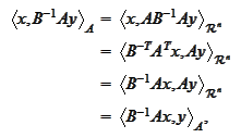
However, it is self-adjoint and positive definite with respect to
 :
:

 Therefore, it has all the necessary spectral properties and we can still apply
the procedure (
Conjugate gradients
).
Another possibility is to try
factorization
 Such decomposition always exists (but not unique) if
 is symmetric positive definite. We
have
 We make the
change
 multiply by
 and arrive
to
 Note that (by similar calculation)
 The matrix
 is symmetric positive-definite in
 .
The procedure (
Conjugate gradients
) then
can be adapted for the equation
 with usual tricks to keep down the number of matrix multiplications.
|