e proceed to extend
results of the sections
(
Vanishing
moments for biorthogonal wavelets
) and
(
Vanishing moments of
wavelet
) to Sobolev spaces
 ,
see the chapter (
Sobolev spaces
). The
section (
Construction
of approximation spaces
) is important prerequisite.
,
see the chapter (
Sobolev spaces
). The
section (
Construction
of approximation spaces
) is important prerequisite.
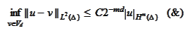
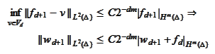
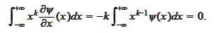
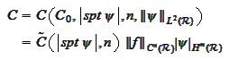
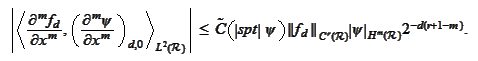
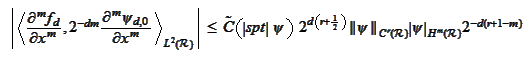
Note
that
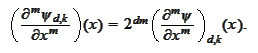
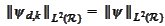
|
|
(Derivative vs scale)
|
Proof
First, we prove the result for
 on
on
 :
:
The method of the prove is assume that
 does not hold and arrive to contradiction using the proposition
(
Vanishing moments vs
approximation 3
). If
does not hold and arrive to contradiction using the proposition
(
Vanishing moments vs
approximation 3
). If
 does not hold then there exists an increasing sequence
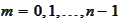
 ,
,
 such
that
such
that
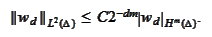
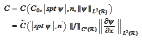
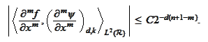
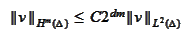
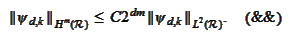
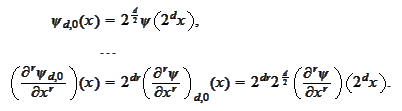
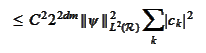
Note that the scale operation does not alter the
 -norm,
see the formula (
Property of
scale and transport 2
), hence we only need to estimate the numerator of
-norm,
see the formula (
Property of
scale and transport 2
), hence we only need to estimate the numerator of
 to show that, in fact, LHS of
 cannot blow up.
In context of the proposition
(
Vanishing moments vs
approximation 3
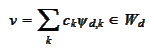
) we take the sequence
 ,
,
 then
then
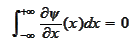
 Note
that
Note
that
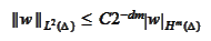
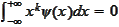
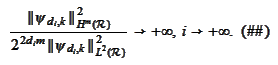
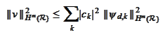
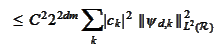
 Thus, for
 to
to
 -approximate
the
-approximate
the
 the
the
 max-norm has to grow like
 :
:
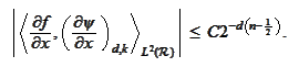
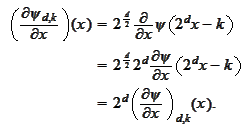
 We also use the formula (
Derivative vs
scale
):
We also use the formula (
Derivative vs
scale
):
 or
or
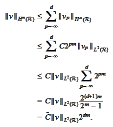
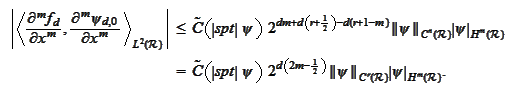 This estimate is in contradiction with
 ,
thus,
,
thus,
 is proven.
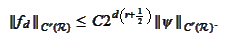
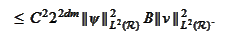
We extend the estimate to
 as follows.
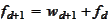
Let
as follows.
Let
 then
then
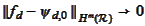
 We apply
 .
.
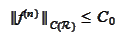
 The
The
 is a
is a
 -constant:
 .
.
 We use the proposition (
Frame property
2
).
We use the proposition (
Frame property
2
).
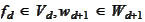
Next, we extend the result to
 .
Let
.
Let
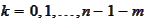
 ,
,
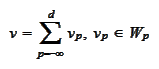 then
then
We have proven the estimate in case of
 .
.
To extend the result to
 we note that the procedure in the section
(
Construction
of MRA and wavelets on half line or an interval
) is a finite linear
combination taken within
we note that the procedure in the section
(
Construction
of MRA and wavelets on half line or an interval
) is a finite linear
combination taken within
 .
.
|