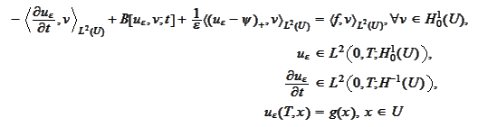
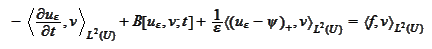
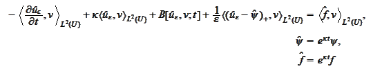
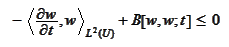
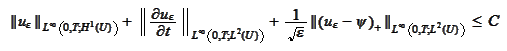
(Evolutionary penalized problem)
For a bounded set
with smooth boundary, time interval
and given functions
,
find a function
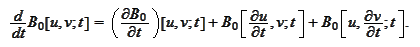
satisfying the relationships
where the operation
is given by the definition (
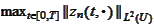
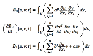
Bilinear form B
2
).
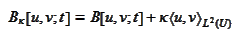
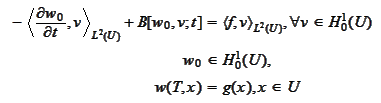
(Existence) We define
to be the solution
of
and define the sequence
as
follows
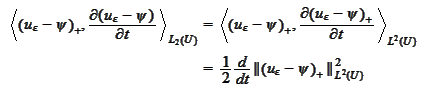
We denote
and derive from
:
We add and
obtain
or
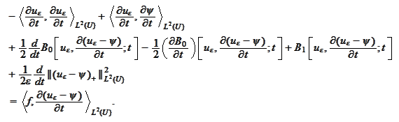
We integrate both sides over
:
or
Note that
hence
Therefore
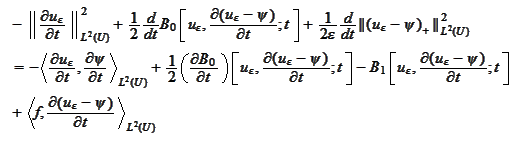
Let
is the point where the
(or we would modify the argument for a sequence that approaches the
).
Then considering
at
we
obtain
Thus
or
Thus, for
sufficiently
small
But then, using such result
and
we increase the
and expand it to
.
Thus
for some
.
Then from
we also
conclude
Then
implies that
and by passing
to the limit,
is the solution of the problem
(
Evolutionary penalized
problem
).
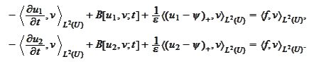
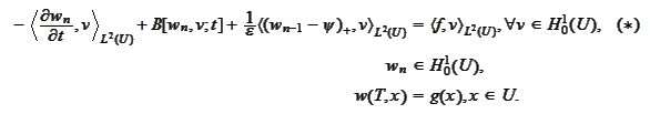
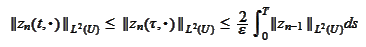
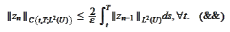
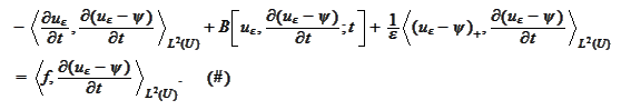
We act similarly to the proof of the proposition
(
Parabolic regularity 1
). We deduce
from the equation of the problem
(
Evolutionary penalized
problem
):
Note that we used the condition
on
of the proposition
(
Existence and
uniqueness for evolutionary problem
) so that
).
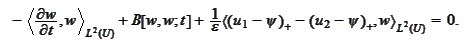
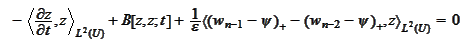
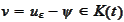
We introduce the following convenience
notations
so
that
We
have
By the condition (
Symmetric principal
part
)
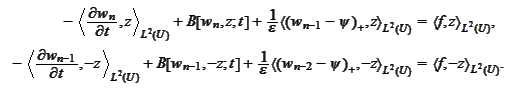
We substitute
,
and
into
:
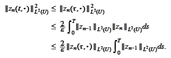
We move the terms
around
and integrate over
.
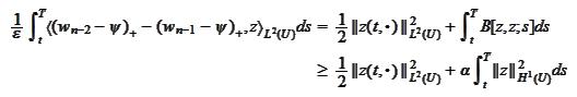
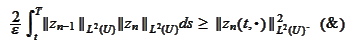
Then, similarly to the proof of the proposition
(
Parabolic regularity 1
), the
-term
estimates from below by ellipticity, all the RHS estimates from above and we
obtain the statement of the proposition.


![$\left[ 0,T\right] $](graphics/notesCF__1__8482.gif)


![$\left[ t,T\right] $](graphics/notesCF__1__8512.gif)


![$\left[ 0,T\right] $](graphics/notesCF__1__8531.gif)


![$\left[ t,T\right] $](graphics/notesCF__1__8558.gif)
