onsider a market consisting of a single stock and a money market account
(MMA). The MMA is riskless and has rate
 .
The price of the stock is given by a stochastic process
 .
At present moment
 the stock is priced at
 .
There is no trading or price evolution until a time moment
 ,
,
 and at
 the stock may assume only two possible prices:
 and
and
 .
Hence, we introduce the random
events
 We would like to come up with a
 -price
for a contract that pays at time
 a random
amount

Suppose that at the moment
 we sell the contract for a price
 ,
purchase
 shares of the stock and put the remainder of the funds
 into the MMA. Any of the values
 may be negative. We assume that we can short the stock and borrow from MMA at
the same rate
 .
.
The value of the position
 is
zero:
 We hold the position until the time moment
 when there are two
possibilities:
 Let us select
 and
and
 so that
 would be the same for both
situations:

 We arrive to a system
 of two
equations:
 The
quantity
 is called "delta" and the strategy of taking position in the underlying stock
equal to
 is called "delta hedging".
To determine
 we make the following "no arbitrage" argument. At
 we have a position of zero value. At the moment
 we have a position of set value (given our selection of
 ).
Such set value has to be zero because otherwise we made or lost money in
absence of risk, hence, the price
 of the contract would not be correct. Therefore, we have a third
equation:
 from which we derive
 :
:
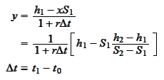
 and we obtain the correct price of the contract:
 We would like to put the above result into the
form
 for some numbers
 .
Hence, we rearrange the expression
 :
:
 thus
thus
 Note
that
 For this reason we call the numbers
 the "risk neutral
probabilities":
 and represent the expression
 as the "risk neutral expectation of discounted
payoff":

|