et
 be a
space-direction finite difference operator,
be a
space-direction finite difference operator,
 Assume that
 is independent from
 .
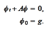
We seek for efficient ways to convert to a finite difference scheme in
.
We seek for efficient ways to convert to a finite difference scheme in
 -direction.
We integrate over
-direction.
We integrate over
 :
:
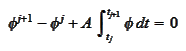 and approximate the
integral
and approximate the
integral
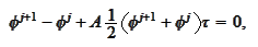 where the
 is the step
 .
Hence,
.
Hence,
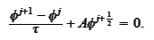
 If the operator
 is positive definite the the norm of
 is less then
 and the scheme is stable.
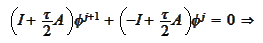
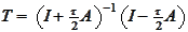
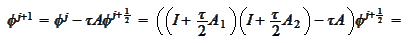
The predictor-corrector way to improve scheme's efficiency is the following.
We find a separation
 for the implicit part of the scheme. Observe that the Crank-Nicolson may be
written in two steps as
for the implicit part of the scheme. Observe that the Crank-Nicolson may be
written in two steps as
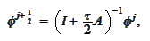
 We transform
further
We transform
further


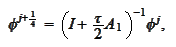
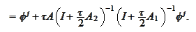
 The last equation is equivalent
to
The last equation is equivalent
to
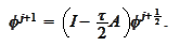
 We aim to replace the last equation with the
equation
We aim to replace the last equation with the
equation
 To see that we preserve the second order of approximation we
compute
To see that we preserve the second order of approximation we
compute
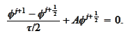
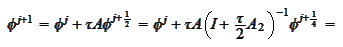
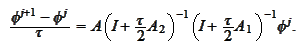
 The resulting scheme is
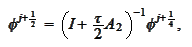
 These should be more efficient because we split the inversion into two,
presumably, simpler components. The last step is explicit.
These should be more efficient because we split the inversion into two,
presumably, simpler components. The last step is explicit.
To explore stability we put all steps
together
 Hence
Hence
 Make the change of
function
Make the change of
function
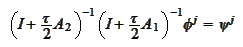 then
then
 and the stability follows from the stabilization scheme considerations.
|
