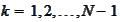
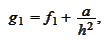
onsider the
following boundary
problem:
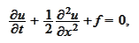
 where the
 is the unknown function, the functions
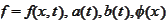 are given and regular, and the variable
 and
and
 lie in the domain
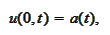
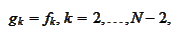
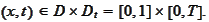 We set up the lattice
 and approximate
 with the
 .
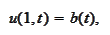
We arrive to the following ODE
problem
.
We arrive to the following ODE
problem


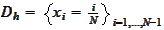
 for
for
 ,
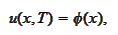
where
,
where
 ,
,
 ,
,
 .
.
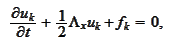
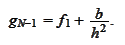
Let us consider the boundary conditions. The matrix of the Laplacian
 has the
form
has the
form
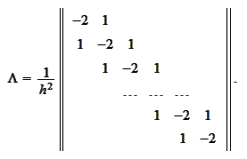 Note what happens to the finite difference approximation of the second
derivative on the edges of the matrix. Obviously, we do not approximate it if
Note what happens to the finite difference approximation of the second
derivative on the edges of the matrix. Obviously, we do not approximate it if

 are some non zero values. We perform the following trick. We
set
are some non zero values. We perform the following trick. We
set
 Then the
equation
Then the
equation
 will describe exactly the same
 if we choose
 according
to
according
to
|
|
(Boundary trick)
|
 Set up the lattice
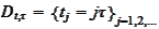 covering the
 and integrate the
 -th
equation over the interval
-th
equation over the interval
 .
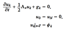
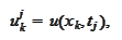
We
have
.
We
have
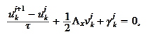 where
where
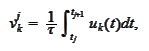
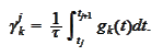 The integral may be approximated by one of the quadrature
formulas
The integral may be approximated by one of the quadrature
formulas
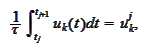
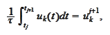
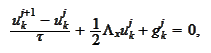
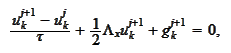
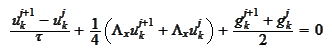
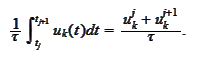 The resulting schemes are called implicit, explicit and Crank-Nicolson schemes
respectively. The expressions for the schemes
are
The resulting schemes are called implicit, explicit and Crank-Nicolson schemes
respectively. The expressions for the schemes
are
|
|
(Implicit scheme)
|
|
|
(Explicit scheme)
|
|
|
(Krank Nicolson)
|
with the boundary
conditions
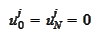 in every case.
|
