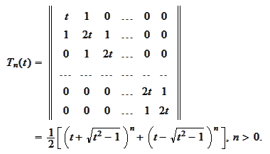
(Chebyshev polynomials) Chebyshev
polynomials
are deduced from the
rule
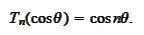
Note that
.
The particular normalization
is denoted
,
.
Proposition
(Trigonometry
primer)
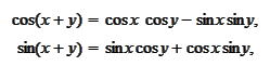
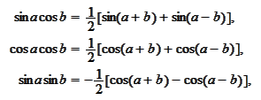
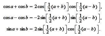
Proposition
(Chebyshev polynomials
calculation) We
have
In
particular,
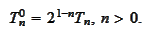
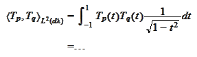
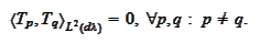
Proposition
(Chebyshev polynomials
orthogonality) Chebyshev polynomials are orthogonal with respect to the
measure
:
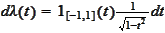
Proof
We verify orthogonality
directly:
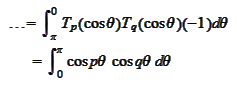
We make the change
,
,
,
for
,
.
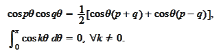
Note that
Thus
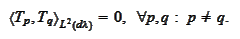
Proposition
(Minimum norm
optimality of Chebyshev polynomials) We
have
Proof
Because
the polynomial
alternates between its minimal value
and maximal value
on the interval
and achieves each extremum
times on
.
Assume that there exists a
such that
.
Then
changes sign
times and, thus, has
zeros. But
and cannot have
zeros.