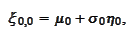
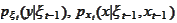
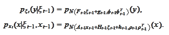
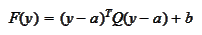
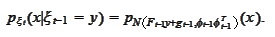
e are considering equations of the
form
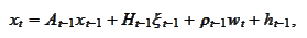
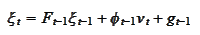 where
where
 are known time dependent deterministic matrixes,
 is observable at time
 random quantity,
 is a non observable random quantity that realized (determined) itself at
 ,
,
 and
and
 are vectors of iid standard normal variables, realized at time
 and
and
 are known deterministic vectors. We will say that
 is the the observable part of the information and the
 is the total description at time
 .
.

We start at time
 .
We are given the distribution
.
We are given the distribution
 and
and
 .
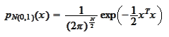
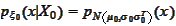
We assume that the distribution for the
.
We assume that the distribution for the
 is normal:
 where the
 is a vector of
 -measurable
iid standard normal variables.
-measurable
iid standard normal variables.
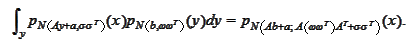
We will be repeatedly using the following result (see
(
Linear transformation
of random variables
)).
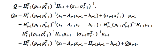
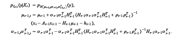
The summary of the procedure is as follows. We have the distribution
 from previous steps and
 from
the model. We calculate
from
the model. We calculate
 through steps
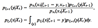 The
The
 is the normalization term. We do not need to calculate it explicitly. The
distributions
is the normalization term. We do not need to calculate it explicitly. The
distributions
 come from the model.
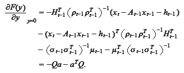
 The integral is calculated using the result of the previous
section:
The integral is calculated using the result of the previous
section:
We have
 for
for
 .
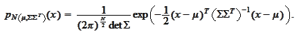
We calculate
.
We calculate
 with precision up to a multiplicative normalization
constant:
with precision up to a multiplicative normalization
constant:
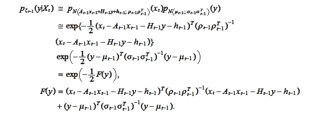 We would like to put
 to the
form
to the
form
 for some symmetrical
 .
We are interested only in the knowledge of
.
We are interested only in the knowledge of
 and
and
 .
Hence,
.
Hence,
 Therefore,
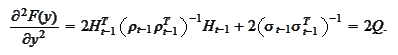
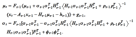
 The
The
 is the inverse of the result's covariance matrix. We calculate it as follows
 Using one of the forms for
 above we calculate
 as
follows
as
follows
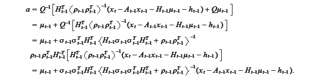 We
conclude
We
conclude
Following the outlined procedure we now
calculate
 where the
 we have just obtained and the
 comes from the
model
comes from the
model
 Hence, we apply the formula for the convolution of normal
distributions
Hence, we apply the formula for the convolution of normal
distributions
 We
have
We
have
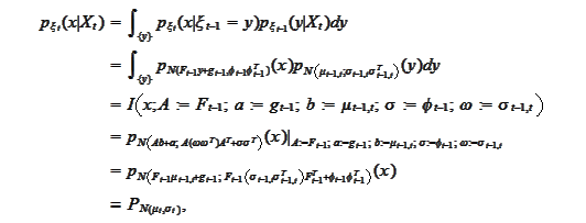
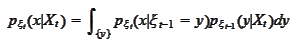
 The recursion is completed.
|